Music Recommendation System

In this post, I will be documenting my journey in creating a recommendation system from scratch using my music that I have collected from Spotify. This post will be divided into two parts:

1. Data Collection
2. Model Training
3. Evaluation
4. Conclusion

Before we go further, I think it’s important to know what is NMF, how NMF works, and why I chose this algorithm to create a recommendation system.

What is NMF?

Non-negative Matrix Factorization (NMF) is a matrix factorization method that factorizes a non-negative matrix into two non-negative matrices. NMF equation can be expressed as follows:

where:

• $V$ is a matrix of song attributes.
• $W$ is a matrix of the latent space.
• $H$ is a matrix of the latent features.
• $n$ is the number of songs.
• $m$ is the number of features.
• $p$ is the number of latent features.

The goal of NMF is to find the latent features and the coefficients of the latent features that can reconstruct the original matrix. Note that the latent topics in $p$ are not directly observable in the data but are inferred from the relationships between songs and their attributes.

How do we determine if a song is similar to other songs? First, we are going to feed matrix $V_{n \times m}$ into the NMF algorithm from scikit-learn with $p$ latent features that produces $W_{n \times p}$. Assuming that we have a song with $p$ features, let’s call it $S = [s_1, ..., s_p]$. Once we have matrix $W$, we can multiplicate it with $S^T$. Thus, $W \times S^T$ will give us a vector $R$ containing values representing how similar the song is to other songs, ranging from 0 to 1. $0$ represents that the song is not similar to a particular song. Conversely, $1$ represents that the song is very similar to a particular song.

Now we know what NMF is and how it works in mathematical perspective. Here are the reasons why I chose NMF as the algorithm behind my music recommendation system:

1. NMF can be scaled to large datasets, which is essential for music services that have vast amounts of tracks and user data.
2. NMF models can be updated incrementally with new data (new users or new songs), which is crucial for dynamic systems like music recommendation services where the database is constantly growing
3. Just like other matrix factorization techniques, NMF reduces the dimensionality of the feature space. This is beneficial because it helps in handling the curse of dimensionality and noise in the data. In the reduced space, similar songs are closer to each other, making it easier to find and recommend similar items.

Data Collection

Since I am a Spotify subscriber, I use their public APIs to collect approximately 2000 songs both from my own playlists and other playlists that I have never listened to. If you’re interested on how I collected the data, you check the script here on GitHub.

There are endpoints that I used to collect the metadata of songs in my own playlist and also songs in the playlists that I never listened to:

1. https://accounts.spotify.com/authorize to get the access token
2. https://accounts.spotify.com/api/token to get the refresh token
3. https://api.spotify.com/v1/me/playlists to get all of my playlists
4. https://api.spotify.com/v1/browse/categories/{category_id}/playlists to get all of the playlists in a category
5. https://api.spotify.com/v1/playlists/{playlist['id']}/tracks to get all of the tracks in a playlist
6. https://api.spotify.com/v1/tracks?ids={track_ids} to get the tracks’ metadata in a bulk
7. https://api.spotify.com/v1/audio-features?ids={track_ids} to get the tracks’ audio features in a bulk

While gathering the data, make sure that you send a request and get the response in a bulk. This way, you can reduce the number of requests that you send to the API. Spotify API has a rate limit of 10 requests per second, so you have to be careful when sending requests to the API.

Here is one of the songs’s metadata that the API returns:

1
{
2
  "id": "2i2gDpKKWjvnRTOZRhaPh2",
3
  "title": "Moonlight",
4
  "artist(s)": "Kali Uchis",
5
  "popularity": 88,
6
  "danceability": 0.639,
7
  "energy": 0.723,
8
  "key": 7,
9
  "loudness": -6.462,
10
  "mode": 0,
11
  "speechiness": 0.0532,
12
  "acousticness": 0.511,
13
  "instrumentalness": 0.0,
14
  "liveness": 0.167,
15
  "valence": 0.878,
16
  "tempo": 136.872,
17
  "type": "audio_features",
18
  "uri": "...",
19
  "track_href": "...",
20
  "analysis_url": "...",
21
  "duration_ms": 187558,
22
  "time_signature": 4
23
}

To understand the meaning of each feature, you can read the documentation here. While writing this post halfway, I stumbled upon a library called Spotipy that can be used to interact with Spotify API. I could have used this library to collect the data, but I decided to stick with my own script.

Data Exploration

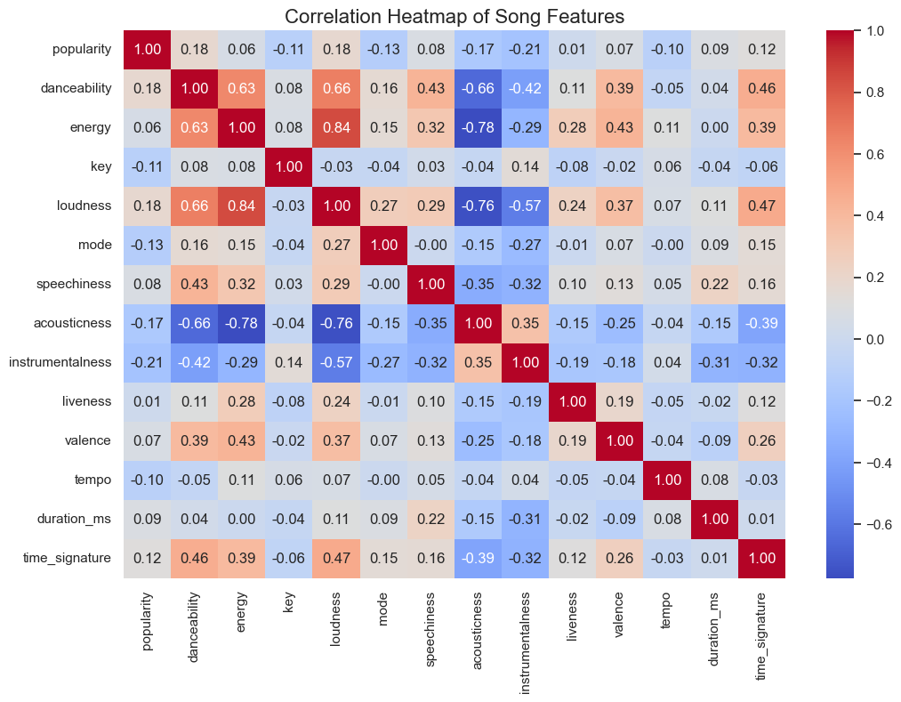
Looking at the heatmap above, we can see danceability, energy, and loudness are highly correlated. Let’s see how the distribution of each feature looks like.

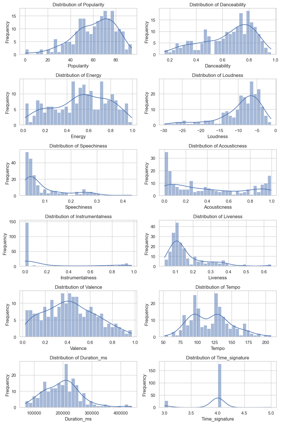
From the distribution above, we can see that most of the songs in my playlists are popular, danceable, and loud. I assume that’s the reason why the heatmap above shows that those three features are highly correlated.

Things we can notice from the scatter plots above:

1. Most danceable songs are popular.
2. Danceability is positively correlated with energy and loudness.
3. Danceable songs are low in speechiness.
4. Danceability is negative correlated with acousticness and instrumentalness.
5. Danceable songs have quite high tempo.

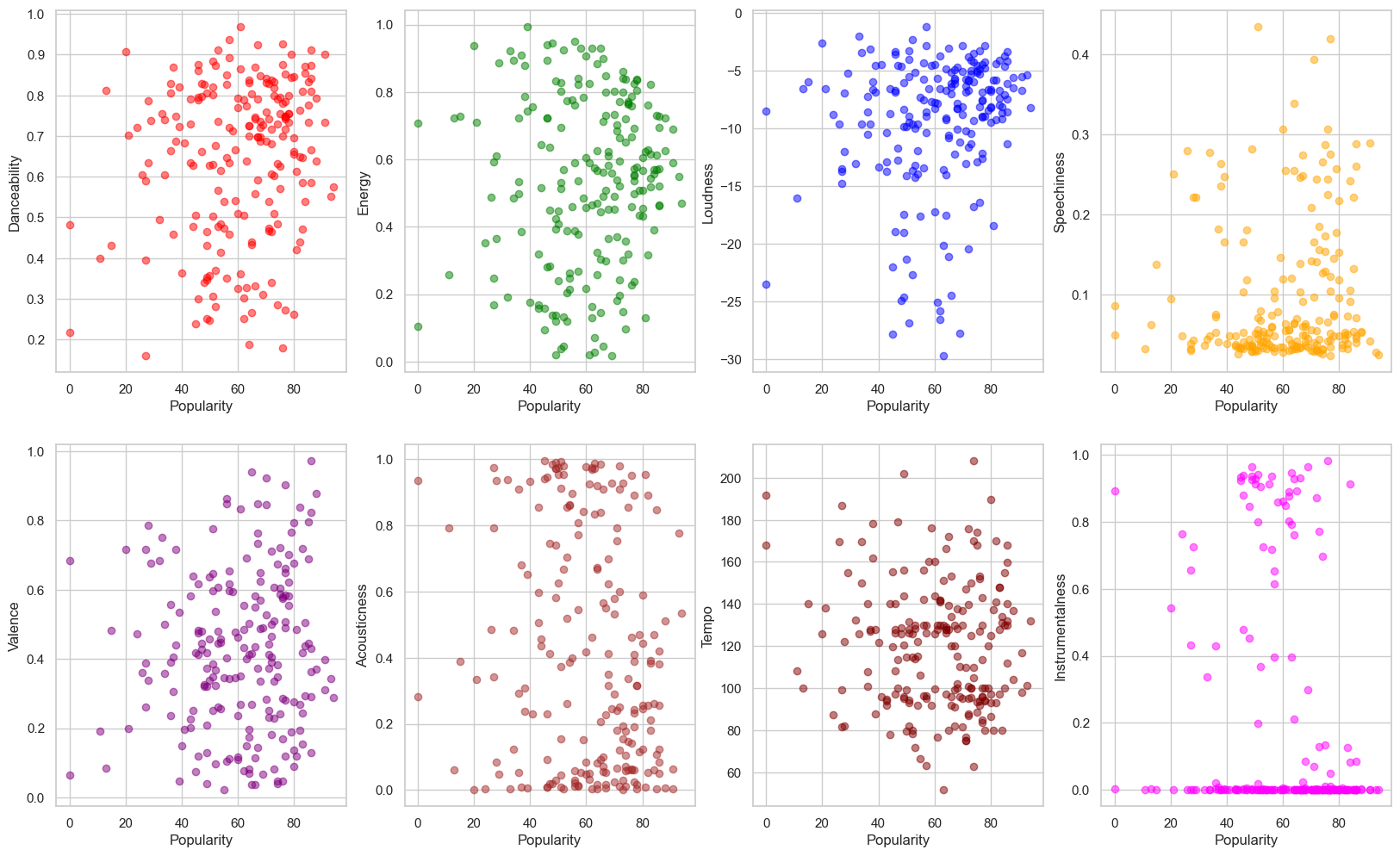
The observations from the scatter plots above:

1. Popular songs are danceable
2. Popular songs are energetic and loud.
3. Popular songs are low in acousticness, instrumentalness, and speechiness.
4. Popular songs are high in valence, meaning that they are happy and cheerful.
5. Popular songs have quite high tempo.

Now let’s see how the data values look like real close. Here is the first 5 rows of the dataset that I converted to a Pandas dataframe:

Let’s see how much each feature contributes to the cumulative variance of the dataset. First we create two lists, one to store the reconstructed errors and the other to store the number of dimensions, starting from 2 to the number of columns in the dataset.

1
reconstruction_errors = []
2
dimensions = range(2, df.columns.size + 1)

After that, we create a pipeline that will scale the data, perform NMF, and normalize the data. Then we fit the pipeline to the dataset and append the reconstruction error to the list so that we can plot it.

1
# create an elbow plot to determine the optimal number of dimensions
2
for dimension in dimensions:
3
  pipeline = make_pipeline(
4
    MinMaxScaler(),
5
    NMF(
6
      n_components=dimension,
7
      max_iter=10000,
8
    ),
9
    Normalizer()
10
  )
11

12
  pipeline.fit(df)
13

14
  reconstruction_errors.append(
15
    pipeline.named_steps['nmf'].reconstruction_err_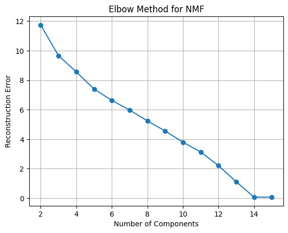
16
  )

The general rule of thumb is to choose the number of components where the elbow starts to flatten out. However, the reconstruction error above has a step decline and only flattens out at 14 dimensions. Now, two questions emerged:

1. Should I use all of the features to create a better recommendation system? That’s where the reconstruction error flattens out.
2. Should I just use half the number of the features to create a so-so recommendation system?

Looking at the graph, I was tempted to use all of the features to create the “perfect” recommendation system. However, there is a catch. If I use all of the features, meaning that the recommendation system will be so good that it will recommend me songs that I have already listened to.

Therefore, if I want to create a recommendation system that will recommend me songs that I have never listened to, I have to use half the number of the features to allow some mistakes to happen. Those mistakes will expose me to new songs or new genres that I have never listened to.

Model Training

This time, let’s use 7 dimensions to create a recommendation system, and get the names of those 7 features.

1
pipeline = make_pipeline(
2
  MinMaxScaler(),
3
  NMF(
4
    n_components=dimension,
5
    max_iter=10000,
6
  ),
7
  Normalizer()
8
)
9
transformed_songs = pipeline.fit(df)
10

11
components = pipeline.named_steps['nmf'].components_
12

13
categories = pd.DataFrame(components, columns=df.columns.values)

There are two variables that we need to pay attention to, which are transformed_songs and categories. First, let’s look how categories looks like:

Each row represents a feature. For example, the 1st feature is popularity since the first colums has the maximum value. This applies to the other rows, meaning other feature.

The discovered categories are:

1. Popularity
2. Mode
3. Instrumentalness
4. Key
5. Speechiness
6. Valence
7. Acousticness

Evaluation

If we print out the first element of transformed_songs, we will get something like this:

1
array([0.68781855, 0.        , 0.02267717, 0.42057155, 0.03739232,
2
       0.46179948, 0.36722474])

Let’s present those values in a dataframe:

1
column_names = ["popularity", "mode", "instrumentalness", "key", "speechiness", "valence", "acousticness"]
2

3
transformed_songs_df = pd.DataFrame(
4
  transformed_songs,
5
  index=no_dup_songs['title'],
6
  columns=column_names
7
)

transformed_songs_df would look nicer like this:

We can make it even nicer by categorizing each song based on the most dominant feature. First we gotta get the index of the dominant category.

1
dominant_categories = [np.argmax(processed_songs.iloc[i]) for i in range(len(processed_songs))]

Then we create a new dataframe using the dominant_categories and get the name of the category using the index.

1
categorized_songs = pd.DataFrame(
2
  [categories.iloc[i].sort_values(ascending=False).index.values[0] for i in dominant_categories],
3
  index=no_dup_songs.title,
4
  columns=["categories"]
5
)

Here is the first 20 rows of the categorized songs:

Just by looking at the first 20 rows, I can say that the model does a pretty good job at categorizing the songs. Counting the number of songs in each category, I noticed most songs I like and listen to are popular songs.

1
categories
2
popularity          113
3
mode                 33
4
instrumentalness     23
5
key                  17
6
acousticness         14
7
valence               7
8
speechiness           1

Take a music called “Idea 1” for example. It is an piano instrumental music that I often listen to. Let’s see what the model would recommend me based on that song.

1
wanted_song = processed_songs.loc['Idea 1']
2
recommended_songs = processed_songs.dot(wanted_song)

Looking at the recommended songs below, I think the model did an impressive job since most of the songs are instrumental songs that in the same genre as “Idea 1”.

To test the model, let’s use the music that I have never listened to before.

Just by listening to these twenty songs, I notice that mose of them have a lot of instrumental elements, pretty much similar to “Idea 1”.

Conclusion

In this project, I have successfully created a decent recommendation system that can recommend me songs using Non-negative Matrix Factorization (NMF). Other than this technique, there are other algorithms that can be used to create a recommendation system, such as Singular Value Decomposition (SVD), Alternating Least Squares (ALS), and Collaborative Filtering (CF). However, I chose NMF because it was the algorithm that I have never heard about until I was reading my old notes from my Linear Algebra class.

Am I satisfied with the result? Yes, I am, and it really help me discovered new songs that I have no idea about, and a lot of them ended up in my own playlists.

References

1. D. Lee, Daniel. Seung, H. Sebastian. (1999). Learning the parts of objects by non-negative matrix factorization. Nature. 401. 788-791. https://www.nature.com/articles/44565.
2. Wikipedia. Non-negative matrix factorization. https://en.wikipedia.org/wiki/Non-negative_matrix_factorization.