Convolutional Neural Networks

Neural Networks: 6 Part(s)

Introduction

Convolutional Neural Network (CNN) is a class of deep Neural networks that mostly utilized for detecting objectts and patterns in images. It was first introduced by Yann LeCun¹ in 1998.

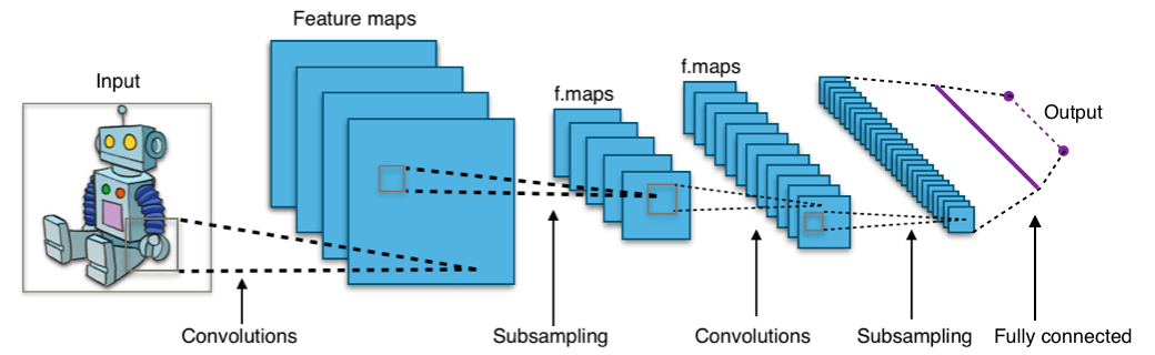Layers in Convolutional Neural Network (Source: Wikipedia)

CNNs consist of:

Convolutional layer is the core building block of CNN. This layer consists of filters, known as kernels or feature maps, which contain features of input images. Higher layers of the network contains more abstract and complex features, such as shapes an patterns. Deeper layers of the network contains simpler features, such as edges and corners.
Pooling layer is used to simplify the spatial dimensions of the Convolutional layer.
Fully connected layer is the layer that performs high-level reasoning and decision making.
Output layer is the final layer which contains units that correspond to the number of classes in the dataset.

Implementation of CNN

In this implementation, we are going to use the Chest X-Ray Images² from Kaggle to detect the presence of pneumonia in x-ray images.

Machine Specifications

OS: Ubuntu 20.04 LTS
CPU: AMD Ryzen 7 3700X
GPU: NVIDIA GeForce RTX 4090 24GB
RAM: 64GB DDR4

Keras

Before going deeper, please refer to the setting up Tensorflow environment post so we could create a separate environment and avoid any compatibility issues.

Let's define the CNN model using Sequential from Keras.

height, width = 224, 224
 
model = Sequential([
  Conv2D(32, (3, 3), activation='relu', input_shape=(height, width, 3)),
  MaxPooling2D((2, 2)),
  Conv2D(64, (3, 3), activation='relu'),
  MaxPooling2D((2, 2)),
  Conv2D(128, (3, 3), activation='relu'),
  MaxPooling2D((2, 2)),
  Flatten(),
  Dense(128, activation='relu'),
  Dense(1, activation='sigmoid')
])
 
model.compile(
  optimizer='adam',
  loss='binary_crossentropy',
  metrics=['accuracy']
)
 
model.summary()

This is what we would get:

Model: "sequential"
_________________________________________________________________
Layer (type)                 Output Shape              Param #
=================================================================
conv2d (Conv2D)              (None, 222, 222, 32)      896
_________________________________________________________________
max_pooling2d (MaxPooling2D) (None, 111, 111, 32)      0
_________________________________________________________________
conv2d_1 (Conv2D)            (None, 109, 109, 64)      18496
_________________________________________________________________
max_pooling2d_1 (MaxPooling2)(None, 54, 54, 64)        0
_________________________________________________________________
conv2d_2 (Conv2D)            (None, 52, 52, 128)       73856
_________________________________________________________________
max_pooling2d_2 (MaxPooling2)(None, 26, 26, 128)       0
_________________________________________________________________
flatten (Flatten)            (None, 86528)             0
_________________________________________________________________
dense (Dense)                (None, 128)               11075712
_________________________________________________________________
dense_1 (Dense)              (None, 1)                 129
=================================================================
Total params: 11,169,089
Trainable params: 11,169,089
Non-trainable params: 0
_________________________________________________________________

The model consists of 3 Convolutional layers with 3 MaxPooling layers. Let's explain what each layer consists of.

Conv2D(32, (3, 3), activation='relu', input_shape=(height, width, 3)) consists of $32$ filters, or feature maps, with a size of $3 \times 3$ , stride of $1$ , and padding of $0$ . Thus, the output shape would be $222 \times 222 \times 32$ .

MaxPooling2D((2, 2)) reduces the spatial dimensions of the Convolutional layer by $2$ . Thus, the output shape would be $111 \times 111 \times32$ .

Conv2D(64, (3, 3), activation='relu') consists of $64$ filters with a size of $3 \times 3$ . The output shape would be $109 \times 109 \times 64$ .

MaxPooling2D((2, 2)) reduces the spatial dimensions of the Convolutional layer by $2$ . Thus, the output shape would be $54 \times 54 \times 64$ .

Conv2D(128, (3, 3), activation='relu) consists of $128$ filters with a size of $3 \times 3$ . The output shape would be $52 \times 52 \times 128$ .

MaxPooling2D((2, 2)) reduces the spatial dimensions of the Convolutional layer by $2$ . Thus, the output shape would be $26 \times 26 \times 128$ .

Flatten() converts the 3D tensor into a 1D tensor. The output shape would be $26 \times 26 \times 128 = 86528$ units.

Once the features are extracted and flattened, we pass them to the Fully Connected layer. From here, the model performs high-level reasoning and decision making. Once done, the ouput is passed to the Output layer. Then, we would see if an image is classified as pneumonia or not.

Finally, train the model using the GPU and assign the training history to a variable.

with tf.device('/GPU:0'):
  history = model.fit(train_generator, epochs=10, validation_data=validation_generator)

Worry not. 10 times is enough for a simple model. Even with Nvidia RTX 4090, each epoch still takes 1 minute more or less.

...
Epoch 10/10
loss: 0.0945 - accuracy: 0.9632 - val_loss: 0.1310 - val_accuracy: 0.9375

Evaluating the model using the test dataset.

test_loss, test_accuracy = model.evaluate(test_generator)
val_loss, val_accuracy = model.evaluate(validation_generator)

The testing accuracy is 87%. While the validation accuracy is 75%. However, these values may change every time you run the model.

PyTorch

Coming soon ...

Conclusion

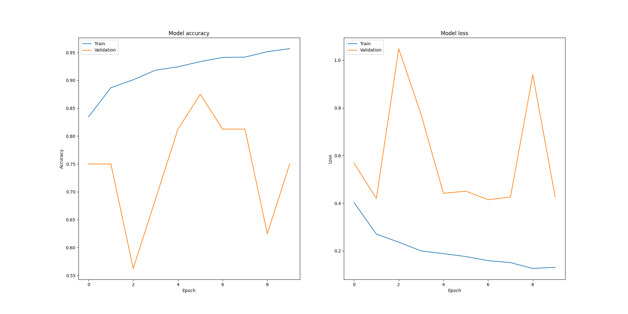Accuracy and Loss of the model

Although from the graph we can see that the validation accuracy is not ideal, this CNN model is relatively simple and good for a start. To improve the model, we could add more Convolutional layers, increase the number of filters, and add Dropout layers to prevent overfitting.

Code

Keras

1. Data Preparation

height, width = 224, 224
batch_size = 32
 
train_datagen = ImageDataGenerator(
  rescale=1./255,
  shear_range=0.2,
  zoom_range=0.2,
  horizontal_flip=True
)
 
test_dataset = ImageDataGenerator(rescale=1./255)
 
train_generator = train_datagen.flow_from_directory(
  os.path.join(data_dir, 'train'),
  target_size=(height, width),
  batch_size=batch_size,
  class_mode='binary'
)
 
test_generator = test_dataset.flow_from_directory(
  os.path.join(data_dir, 'test'),
  target_size=(height, width),
  batch_size=batch_size,
  class_mode='binary'
)
 
validation_generator = test_dataset.flow_from_directory(
  os.path.join(data_dir, 'val'),
  target_size=(height, width),
  batch_size=batch_size,
  class_mode='binary'
)

2. Data Visualization

import matplotlib.pyplot as plt
 
fig, ax = plt.subplots(1, 2, figsize=(20, 10))
ax[0].imshow(train_generator[0][0][0])
ax[0].set_title('Normal X-Ray')
 
ax[1].imshow(test_generator[0][0][0])
ax[1].set_title('Pneumonia X-Ray')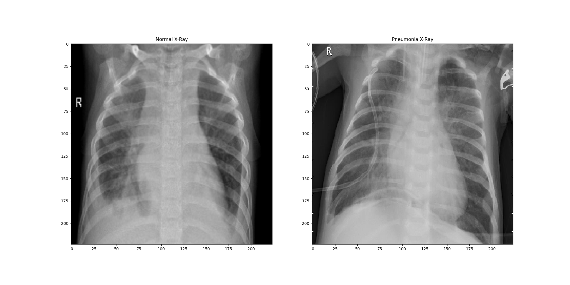

Normal and Pneumonia X-Ray images

3. Model Definition

model = Sequential([
  Conv2D(32, (3, 3), activation='relu', input_shape=(height, width, 3)),
  MaxPooling2D((2, 2)),
  Conv2D(64, (3, 3), activation='relu'),
  MaxPooling2D((2, 2)),
  Conv2D(128, (3, 3), activation='relu'),
  MaxPooling2D((2, 2)),
  Flatten(),
  Dense(128, activation='relu'),
  Dense(1, activation='sigmoid')
])
 
model.compile(
  optimizer='adam',
  loss='binary_crossentropy',
  metrics=['accuracy']
)
 
model.summary()

4. Model Training, Testing, and Evaluation

with tf.device('/GPU:0'):
  history = model.fit(train_generator, epochs=10, validation_data=validation_generator)
 
test_loss, test_accuracy = model.evaluate(test_generator)
print(f'Test accuracy: {test_accuracy:.2f}%')
 
val_loss, val_accuracy = model.evaluate(validation_generator)
print(f'Validation accuracy: {val_accuracy:.2f}%')

PyTorch

Coming soon ...

References

Keiron O'Shea and Ryan Nash. An Introduction to Convolutional Neural Networks
Zewen Li, Wenjie Yang, Shouheng Peng, Fan Liu. A Survey of Deep Convolutional Neural Network Architectures

Yann LeCun, Léon Bottou, Yoshua Bengio, and Patrick Haffner. Gradient-Based Learning Applied to Document Recognition ↩
Paul Mooney. Chest X-Ray Images (Pneumonia) Kaggle Dataset. ↩

Convolutional Neural Networks

Introduction

Implementation of CNN

Machine Specifications

Keras

PyTorch

Conclusion

Code

Keras

1. Data Preparation

2. Data Visualization

3. Model Definition

4. Model Training, Testing, and Evaluation

PyTorch

References

Footnotes