Linear Regression

What is Linear Regression?

Linear Regression is one of many supervised machine learning algorithms, and it is mosly used to predict the value of a continuous variable, as well as to do forecasting. In other words, it can be used:

1. to see if one variable can be used to predict another variable.
2. to see if one variable is correlated or dependent with another variable.

However, Linear Regression also comes with some limitations, such as:

1. It assumes that the relationship between the independent variable and the dependent variable is linear. However, in reality, the relationship between the independent variable and the dependent variable is not always linear.
2. It assumes that the independent variables are not correlated with each other. However, in reality, the independent variables are not always independent.
3. It's sensitive to outliers. Meaning that the presence of outliers can affect the regression line.

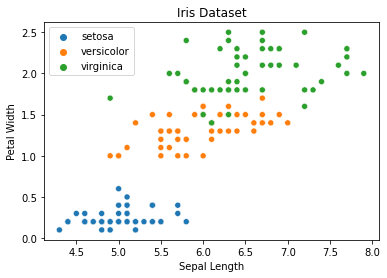
From the graph above, we can see that the relationship between $x$ and $y$ is linear since the blue line starts from the bottom left to the top right. That line is called a regression line, and it can be expressed using the following equation.

where $\theta_0$ is the intercept and $\theta_1$ is the first coefficient. In high school or college, we are used to seeing the equation above in the following form to calculate the distance between one point to another.

In this post, we are going to use two features in the Iris dataset from sklearn-learn, petal width and sepal length. Plotting it will give us the following visualization.

Iris Dataset Scatter Plot

You should know that the intercept or $\theta_0$ is the starting point of the regression line. Whether the line is going up or down depends on the $\theta_1$ and the data. If $\theta_0 = 0$, it means that our regression line will start from $0$.

Expressing the equation like we did above is quite cryptic for people who don't have strong mathematical background. Since we are using the Iris Dataset, we can translate the equation into a more readable form.

From the translation above can tell us the relationship between those two variables. Now you will be wondering their correlations whether sepal_length and petal_width are correlated or inversely correlated. First, let's translate what the two graphs below are trying to tell us.

sepal_length and petal_width are said to be correlated when sepal_length increases, the petal_length also increases. Conversely, sepal_length and petal_width are said to be inversely correlated when sepal_length increases, but the petal_width decreases.

With a regression line, it can help us to predict the $y$ value given a single $x$ value. However, most predictions made by the regression line are not always accurate since its ability to predict depends heavily on $\theta_0$ and $\theta_1$. If the values $\theta_0$ and $\theta_1$ are not tweaked correctly, the regression line will sit right far from most data points.

Estimating the Intercept and Coefficient

Previously, I mentioned that $\hat{y} = \theta_0 + \theta_1x$ is used to express the regression line. To be fair, we can't just look at the data and say, "Ah ha! I can tell that $\theta_0$ is $0$ and $\theta_1$ is $0$." For most of the time, it's not feasible to keep on guessing those values. Thus, it's better to use an iterative method such as Gradient Descent algorithm. What the Gradient Descent algorithm does is to update the $\theta_0$ and $\theta_1$ values based on the cost function and the learning rate.

This example is just a simple linear model, we are going to use the following equations to update intercept and coefficient:

where $\alpha$ is the learning rate, $\theta_p$ is the $p$-th parameter, $J$ is the cost function, and $x_p$ is the $p$-th feature.

Since we only have $\theta_0$ and $\theta_1$, we can simplify the equation above to:

If you are want to know more about Gradient Descent algorithm, you can read the Gradient Descent series here. The series covers the intuition behind Gradient Descent, the math behind it, and its implementation in Python from scratch.

Example

In this section, there will be two examples of regression lines. One with the regression line is far from most data points, and the other one is close to most data points.

Most data points are far from the regression line

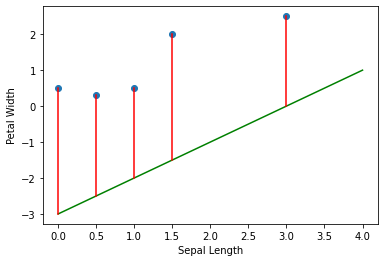
When the regression line, which is indicated by the green line, sees $x = 0$ then it predicts $\hat{y} = -3$. In reality, $y$ should be $0.5$ when $x = 0$. Meaning that the predicted value is far from the actual value.

There are many ways to measure the quality of regression lines, such as:

1. R Squared
2. Mean Squared Error (MSE)
3. Root Mean Squared Error (RMSE)
4. Mean Absolute Error (MAE)

However, we are going to use Mean Squared Error (MSE) this time.

where $n$ is the number of data points, $\hat{y}_i$ is the predicted value, and $y_i$ is the actual value.

Let's calculate the MSE for the graph above with the data points above.

Let's see another example where the data points are close to the regression line.

Most data points are close from the regression line

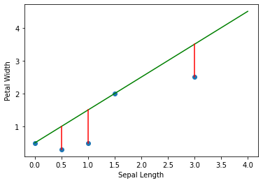
Let's calculate the MSE for this example to see if the MSE is small when the regression line is close to most data points.

From these two examples, we can see that when the regression line is close to most data points, the MSE is small. Conversonly, when the regression line is far from most data points, the MSE is large.

Is having a small MSE enough to say that the regression line is good? Futher investigation is needed to answer this question. However, I am not gonna cover it in this post.

Python Implementation

First prepare the dataset. We are going to use the Iris dataset from sklearn-learn with two features, petal_width and sepal_length.

from sklearn.datasets import load_iris
 
iris = load_iris()
sepal_length = iris.data[:, 0]
petal_width = iris.data[:, 3]
target = iris.target
 
species_dict = {0: 'setosa', 1: 'versicolor', 2: 'virginica'}
species_name = [species_dict[i] for i in target]

Note that, the regression line is calculated using the following equation.

b, x = 0, 0
 
regression_line = [
  b + sepal_length[i] * x for i in range(len(sepal_length))
]

where $\theta_0$ is the intercept and $\theta_1$ is the first coefficient. In this case, we are going to replace $\theta_0$ with b and $\theta_1$ with x. Without any assumption, we are going to start with b=0 and x=0.

sns.scatterplot(x = sepal_length, y = petal_width, hue=species_name)
plt.plot(sepal_length, y, c='r')
plt.title('Iris Dataset: Sepal Length vs Petal Width')
plt.xlabel('Sepal Length')
plt.ylabel('Petal Width')
plt.legend()
plt.show()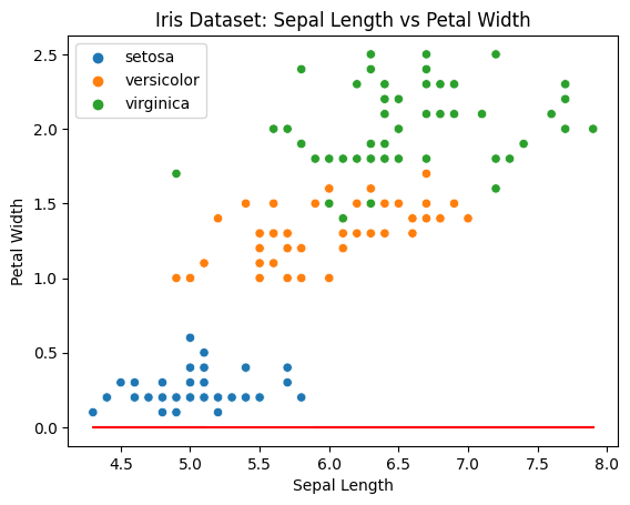

Regression line with b=0 and x=0

Looking at the plot above, we can tell that the regression line is far from most data points. Thus, we need to automatically tweak b and x to get a better regression line using the Gradient Descent algorithm.

def linear_regression(x, y, epochs, alpha = 0.01):
    intercept, coefficient = 0, 0
    length = len(x)
 
    for _ in range(1, epochs):
        predictions = predict(intercept, coefficient, x)
        errors = predictions - y
        # gradient descent algorithm happens here
        intercept = intercept - alpha * np.sum(errors) / length
        coefficient = coefficient - alpha * np.sum(errors * x) / length
        # ends here
        mse_history.append(mean_squared_error(errors))
        intercept_history.append(intercept)
        coefficient_history.append(coefficient)
 
    return intercept, coefficient

After running the Gradient Descent algorithm above for $10,000$ times, we get the following regression line where $b=-2.71$ and $x=0.67$.

Regression line with b=-2.71 and x=0.67

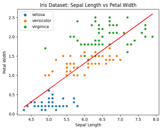
You would notice there are three lists: mse_history, intercept_history, and coefficient_history. I made them just to see how the MSE, intercept, and coefficient change over time.

MSE, Intercept, and Coefficient over time

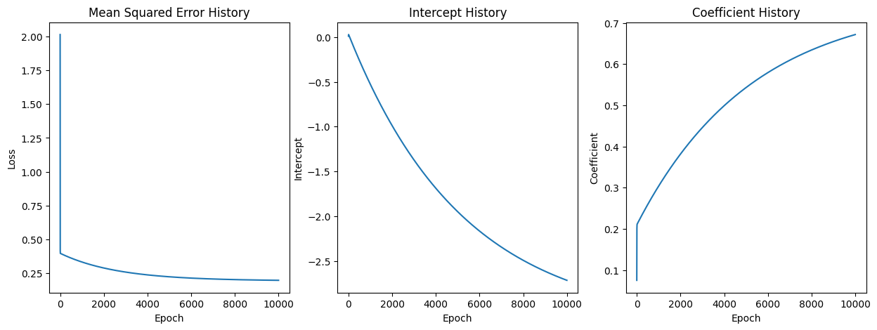
I have also plot the MSE, intercept, and coefficient in the 3D space to see how they change over time.

MSE, Intercept, and Coefficient in 3D space

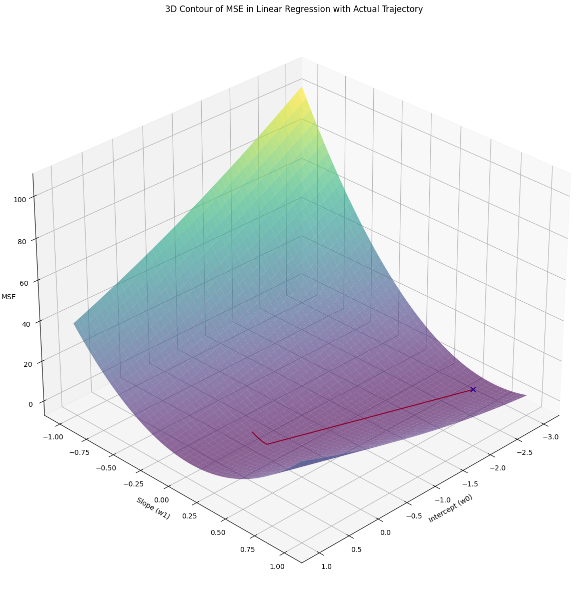
Note that the blue x marks the lowest MSE value calculated with the estimated intercept and coefficient we got from the Gradient Descent algorithm.

To see how I made this graph, you could check out the source code here.

Conclusion

1. Linear Regression is a supervised learning algorithm that is used to predict the value of a continuous variable.
2. The equation of the regression line is $y = \theta_0 + \theta_1 \times x$.
3. The regression line is said to be good when it is close to most data points.
4. The quality of the regression line can be measured using evaluation metrics, one of them is Mean Squared Error (MSE).
5. The smaller the MSE, the closer the regression line is to most data points. Conversely, the larger the MSE, the farther the regression line is to most data points.
6. $b$ and $x$ can be estimated using Gradient Descent algorithm.

Code

Simple Implementation

mse_history = list()
intercept_history = list()
coefficient_history = list()
 
def predict(intercept, coefficient, data):
    return intercept + np.dot(coefficient, data)
 
def mean_squared_error(errors):
    return np.mean(np.square(errors))
 
def linear_regression(x, y, epochs, alpha = 0.01):
    intercept, coefficient = 0, 0
    length = len(x)
 
    for _ in range(1, epochs):
        predictions = predict(intercept, coefficient, x)
        errors = predictions - y
        # gradient descent algorithm happens here
        intercept = intercept - alpha * np.sum(errors) / length
        coefficient = coefficient - alpha * np.sum(errors * x) / length
        # ends here
        mse_history.append(mean_squared_error(errors))
        intercept_history.append(intercept)
        coefficient_history.append(coefficient)
 
    return intercept, coefficient
 
b, x = linar_regression(sepal_length, petal_width, 10000)

Printing b and x will give us -2.717366489030271 and 0.6718570469763597.

You could find the source code here.

Scikit-Learn Implementation

import numpy as np
 
class LinearRegression:
    def __init__(self):
        self.iterations = 10_000
        self.learning_rate = 0.01
        self.intercept = 0
        self.coefficients = None
        self.X = None
        self.y = None
        self.length = 0
        self.loss_history = list()
 
    def _intercept(self):
        return self.intercept
 
    def _coefficients(self):
        return self.coefficients
 
    def _loss_history(self):
        return self.loss_history
 
    def mean_squared_error(self, predictions):
        return np.sum(np.square(predictions - self.y)) / self.length
 
    def predict(self, X):
        return self.intercept + np.dot(X, self.coefficients)
 
    def update_params(self, predictions):
        error = predictions - self.y
        self.intercept -= self.learning_rate * np.sum(error) / self.length
        self.coefficients -= self.learning_rate * (np.dot(self.X.T, error) / self.length)
 
    def fit(self, X, y):
        self.X = np.array(X)
        if len(self.X.shape) == 1:
            # To support 1D data, otherwise
            # self.coefficients = np.zeros(self.X.shape[1]) will fail
            self.X = self.X.reshape(-1, 1)
        self.y = np.array(y)
        self.length = len(self.y)
        self.coefficients = np.zeros(self.X.shape[1])
 
        for _ in range(self.iterations):
            predictions = self.predict(self.X)
            self.update_params(predictions)
            self.loss_history.append(self.mean_squared_error(predictions))
 
lin_reg = LinearRegression()
lin_reg.fit(sepal_length, petal_width)
print(f"intercept: {lin_reg._intercept()}, coefficients: {lin_reg._coefficients()}")

Printing the intercept and the coefficient values will give us: intercept: -2.7174583375849535 and coefficients: [0.67187247].

You could find the source code here.

References

1. Wikipedia. Linear Regression. Linear Regression
2. Wikipedia. Gradient Descent. Gradient Descent