Adadelta

Gradient Descent Algorithm: 11 Part(s)

Introduction

Remember that in Adagrad, we have see that each parameter has its own learning rate. However, the learning rate is rapidly decreasing as the number of iterations increases. This can be a problem because the learning rate can become too small and the model stops learning.

In this post, we will see how Adadelta prevents learning rate decreasing rapidly over time. Instead of inefficiently storing, or summing, all the past squared gradients, Adadelta calculates the average of the decayed past gradients and uses it to update parameters. Most importantly, Adadelta uses no learning rate.

Mathematics of Adadelta

The parameter update rule is expressed as

\Delta \theta_t = - \frac{\text{RMS}[\Delta \theta]_{t-1}}{\text{RMS}[g]_t} \odot g_t

\theta_{t+1} = \theta_t + \Delta \theta_t

where

$\Delta \theta_t$ is the update at time $t$
$\theta_t$ is the parameter at time $t$
$\text{RMS}[\Delta \theta]_{t-1}$ is the root mean square of the updates up to time $t-1$
$\text{RMS}[g]_t$ is the root mean square of the gradients up to time $t$
$g_t$ is the gradient at time $t$

$\text{RMS}[\Delta \theta]_{t-1}$ , the root mean square of parameters up to time $t$ , can be expressed as follows:

\text{RMS}[{\Delta \theta}]_{t-1} = \sqrt{E[\Delta \theta^2]_{t-1} + \epsilon}

where $E[\Delta \theta^2]_{t-1}$ is the mean squared parameter updates up to time $t-1$ .

E[\Delta \theta^2]_{t-1} = \gamma E[\Delta \theta^2]_{t-2} + (1 - \gamma) \Delta \theta_{t-1}^2

E[\theta^2]_{t-2} = \frac{\theta_{t-2}^2 + ... + \theta_0^2}{t-2}

$\text{RMS}[g]_t$ , the root mean square of gradients up to time $t$ , can be expressed as follows:

\text{RMS}[g]_t = \sqrt{E[g^2]_t + \epsilon}

where $E[g^2]_t$ is the mean squared gradients up to time $t$ .

E[g^2]_t = \gamma E[g^2]_{t-1} + (1 - \gamma) g_t^2

E[g^2]_{t-1} = \frac{g_{t-1}^2 + ... + g_0^2}{t-1}

$g_{0,t}$ and $g_{1,t}$ are the gradients of the cost function with respect to the intercept and the coefficient respectively, and can be expressed as follows:

\begin{aligned} g_{0,t} &= \nabla_{\theta_0} J(\theta) \\ &= \frac{\partial}{\partial \theta_0} J(\theta) \\ &= \frac{1}{2} \frac{\partial}{\partial \theta_0} (\hat{y}_i - y_i)^2 \\ &= \hat{y}_i - y_i \end{aligned}

\begin{aligned} g_{1,t} &= \nabla_{\theta_1} J(\theta) \\ &= \frac{\partial}{\partial \theta_1} J(\theta) \\ &= \frac{1}{2} \frac{\partial}{\partial \theta_1} (\hat{y}_i - y_i)^2 \\ &= (\hat{y}_i - y_i)x_i \end{aligned}

Implementation of Adadelta

First, define a function that calculates the root mean square of the values.

def rms(past_values, current_value, momentum=0.9, eps=1e-8):
  average = momentum * np.mean(past_values**2) + (1 - momentum) * current_value**2
  return np.sqrt(average + eps)

Second, calculate the intercept and the coefficient gradients. Notice that the intercept gradient $g_{0,t}$ is the prediction error.

new_intercept_gradient = error
new_coefficient_gradient = error * x[random_index]

Third, we need to determine $\text{RMS}[g]_t$ . Since we have define the function rms() in the beginning, we can calculate the root mean square of the gradients.

coefficient_gradient_rms = rms(df['coefficient_gradient'].values, new_coefficient_gradient)
intercept_gradient_rms = rms(df['intercept_gradient'].values, new_intercept_gradient)

Fourth, we need to determine $\text{RMS}[{\Delta \theta}]_{t-1}$ , and we are going to do the same but we are going to apply the function on the intercept and the coefficients columns.

intercept_rms = rms(df['intercept'].values[:epoch], intercept)
coefficient_rms = rms(df['coefficient'].values[:epoch], coefficient)

Finally, we can update the intercept and the coefficient.

delta_intercept = -(intercept_rms / intercept_gradient_rms) * new_intercept_gradient
delta_coefficient = -(coefficient_rms / coefficient_gradient_rms) * new_coefficient_gradient
 
intercept += delta_intercept
coefficient += delta_coefficient

Conclusion

Pathways of SGD, Adagrad, and Adadelta along the 2D MSE contour.

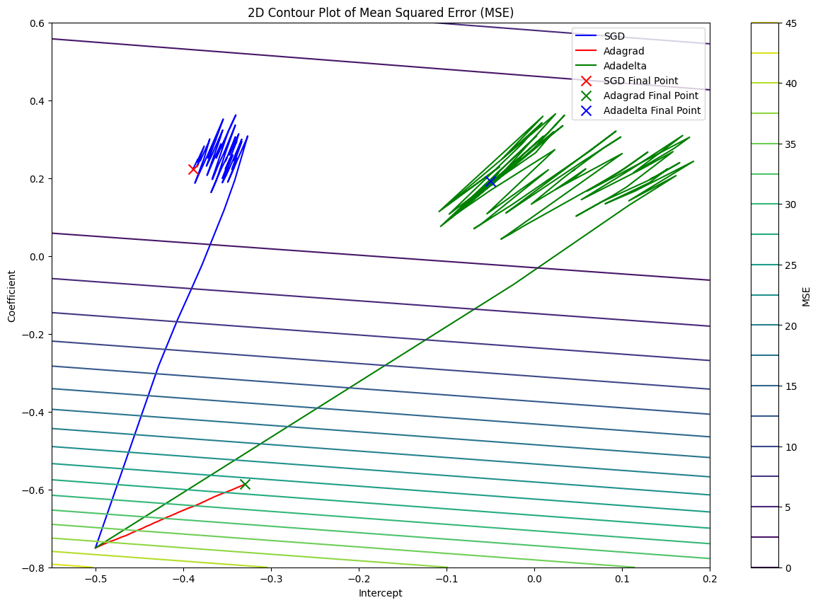
With Adadelta, we can reach the minimum point of the cost function faster than Vanilla SGD and Adagrad. Thus, it allows us to explore more in the parameter space and find the optimal parameters for the model.

Code

def adadelta(x, y, df, epochs=100):
  intercept, coefficient = -0.5, -0.75
  random_index = np.random.randint(len(features))
  prediction = predict(intercept, coefficient, x[random_index])
  error = prediction - y[random_index]
  df.loc[0] = [intercept, coefficient, error, error * x[random_index], (error ** 2) / 2]
 
  for epoch in range(1, epochs + 1):
    random_index = np.random.randint(len(features))
    prediction = predict(intercept, coefficient, x[random_index])
    error = prediction - y[random_index]
 
    new_intercept_gradient = error
    new_coefficient_gradient = error * x[random_index]
 
    intercept_rms = rms(df['intercept'].values[:epoch], intercept)
    coefficient_rms = rms(df['coefficient'].values[:epoch], coefficient)
 
    intercept_gradient_rms = rms(df['intercept_gradient'].values, new_intercept_gradient)
    coefficient_gradient_rms = rms(df['coefficient_gradient'].values, new_coefficient_gradient)
 
    delta_intercept = -(intercept_rms / intercept_gradient_rms) * new_intercept_gradient
    delta_coefficient = -(coefficient_rms / coefficient_gradient_rms) * new_coefficient_gradient
 
    intercept += delta_intercept
    coefficient += delta_coefficient
 
    mse = (error ** 2) / 2
 
    df.loc[epoch] = [intercept, coefficient, new_intercept_gradient, new_coefficient_gradient, mse]
 
  return df

References

Sebastian Ruder. "An overview of gradient descent optimization algorithms." arXiv:1609.04747 (2016).
Zeiler, Matthew D. "ADADELTA: An Adaptive Learning Rate Method." arXiv:1212.5701 (2012).