Stochastic Gradient Descent

Introduction

In the Batch Gradient Descent and Mini-Batch Gradient Descent posts, we have learned that the algorithm updates parameters $\theta_0$ and $\theta_1$ after it has seen the entire dataset and a fraction of the dataset respectively. With these two algorithms, we would need a certain amount of RAM so that the algorithms can converge.

In this post, we are going to learn about Stochastic Gradient Descent, or SGD for short. The only difference between SGD and the other previous algorithms we have covered is that it updates parameters after it has seen a random data point, as the name suggests. Since it only requires a single data point, the need for RAM decreases, and it could help the algorithm converges faster with the least amount of memory.

Mathematics of Stochastic Gradient Descent

The parameter update rule is expressed as

where

• $\theta$ is the parameter vector
• $\alpha$ is the learning rate
• $J(\theta)$ is the cost function
• $\nabla_{\theta} J(\theta)$ is the gradient of the cost function $J(\theta)$

The gradient of the cost function w.r.t. to the intercept $\theta_0$ and the coefficient $\theta_1$ is expressed as the following.

Notice that the gradient of the cost function is the prediction error.

For more details, please refer to the Mathematics of Gradient Descent post.

Implementation of Stochastic Gradient Descent

First, define the predict function.

def predict(intercept, coefficient, x):
  return intercept + coefficient * x

Second, get a random number between 0 and the length of the dataset and predict the value of the random x.

length = len(x)
random_index = np.random.randint(length)
prediction = predict(intercept, coefficient, x[random_index])

Third, determine the error of the prediction and update the intercept $\theta_0$ and the coefficient $\theta_1$.

error = prediction - y[random_index]
intercept_gradient = error
coefficient_gradient = error * x[random_index]

Lastly, update the intercept and the coefficient.

intercept = intercept - alpha * intercept_gradient
coefficient = coefficient - alpha * coefficient_gradient

Conclusion

SGD vs BGD Pathways

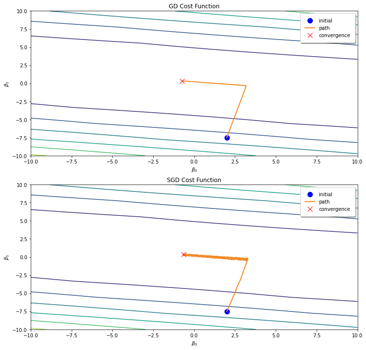
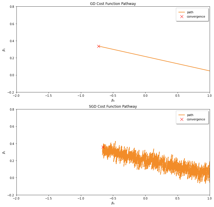
You would notice that the pathway of Vanilla Gradient is much more smoother, and the pathway of SGD is much more thicker than Vanilla Gradient Descent pathway. If we zoom in, we would notice that the SGD pathway is much more noisier.

Zoomed in SGD vs BGD Pathways

There are pros and cons for Vanilla Gradient Descent and SGD. For Vanilla Gradient Descent, it is slow but it is guaranteed to converge to the global minimum. In addition to that, it requires more memory and is not suitable for large dataset since datasets have to be loaded to the RAM before training.

On the otherhand, SGD is faster and is suitable for large dataset since it only requires a single data point to be loaded to the RAM. However, it's not guaranteed to converge to the global minima since it updates parameters $\theta_0$ and $\theta_1$ after seeing a random data point. Not only that, it would struggle to escape local minima and avoid steep regions in the 3D plot of the cost function.

Code

def sgd(x, y, df, epochs, alpha = 0.01):
  intercept, coefficient = 2.0, -7.5
 
  random_index = np.random.randint(len(x))
  prediction = predict(intercept, coefficient, x[random_index])
  error = prediction - y[random_index]
  mse = (error ** 2) / 2
  df.loc[0] = [intercept, coefficient, mse]
 
  for i in range(1,epochs):
    random_index = np.random.randint(len(x))
    prediction = predict(intercept, coefficient, x[random_index])
    error = prediction - y[random_index]
    intercept_gradient = error
    coefficient_gradient = error * x[random_index]
 
    intercept = intercept - alpha * intercept_gradient
    coefficient = coefficient - alpha * coefficient_gradient
 
    mse = (error ** 2) / 2
    df.loc[i] = [intercept, coefficient, mse]
  return df

References

1. Sebastian Ruder. "An overview of gradient descent optimization algorithms." arXiv:1609.04747 (2016)
2. O. Artem. Stochastic, Batch, and Mini-Batch Gradient Descent. https://towardsdatascience.com/stochastic-batch-and-mini-batch-gradient-descent-demystified-8b28978f7f5
3. P. Sushant. Batch, Mini Batch, and Stochastic Gradient Descent. https://towardsdatascience.com/batch-mini-batch-stochastic-gradient-descent-7a62ecba642a
4. Geeksforgeeks. Difference between Batch Gradient Descent and Stochastic Gradient Descent. https://www.geeksforgeeks.org/difference-between-batch-gradient-descent-and-stochastic-gradient-descent/
5. Sweta. Batch, Mini Batch, and Stochastic Gradient Descent. https://sweta-nit.medium.com/batch-mini-batch-and-stochastic-gradient-descent-e9bc4cacd461
6. R. Sebastian. Gradient Descent and Stochastic Gradient Descent. https://rasbt.github.io/mlxtend/user_guide/general_concepts/gradient-optimization/
7. Geeksforgeeks. ML | Mini-Batch Gradient Descent with Python. https://www.geeksforgeeks.org/ml-mini-batch-gradient-descent-with-python/