Batch Gradient Descent

Introduction

In the Mathematics of Gradient Descent, we have discussed what Gradient Descent is, how it works, and how to derive the equations needed to update the parameters of the model.

In this post, we are going to write Batch Gradient Descent from scratch in Python.

Setting Up The Dataset

Throughout this series, we are going to use the Iris Dataset from UCI Machine Learning Repository imported from scikit-learn. There are two features in the dataset that we are going to analyse, namely sepal_length and petal_width shown in the highlighted lines.

from sklearn.datasets import load_iris
 
iris = datasets.load_iris()
features = iris.data
target = iris.target
 
sepal_length = np.array(features[:,0])
petal_width = np.array(features[:,3])
 
species_map = {0: 'setosa', 1: 'versicolor', 2: 'virginica'}
species_names = [species_map[i] for i in target]

Setting Up A Baseline

Before we implement Batch Gradient Descent in Python, we need to set a baseline to compare against our own implementation. So, we are going to train our dataset into the Linear Regression built-in function made by scikit-learn.

First, let's fit our dataset to LinearRegression() model that we imported from sklearn.linear_model.

linreg = LinearRegression()
 
linreg.fit(
    X = sepal_length.reshape(-1,1),
    y = petal_width.reshape(-1,1)
)
 
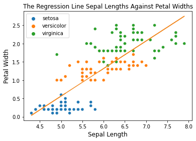
print("Intercept: ",linreg.intercept_[0])
# Intercept: -3.200215
print("First coefficient:", linreg.coef_[0][0])
# First coeficient: 0.75291757

Once we have the intercept and the coefficient values, let's make a regression line to see if the line is close to most data points.

sns.scatterplot(
    x = sepal_length,
    y = petal_width,
    hue = species_names
)
 
plt.plot(
    sepal_length,
    linreg.intercept_[0] +
    linreg.coef_[0][0] * features[:, 0],
    color='red'
)

The iris dataset regression line with Scikit

Clearly, the line is indeed very close to the most data points and we want to see the MSE of this regression line.

linreg_predictions = linreg.predict(sepal_length.reshape(-1,1))
linreg_mse = mean_squared_error(linreg_predictions, petal_width)
print(f"The MSE is {linreg_mse}")
# The MSE is 0.19101500769427357

From the result we got from sklearn, the best regression line is

with MSE value around $0.191$. The equation above is going to be our base line for this experiment to determine how good our own Gradient Descent implementation.

Mathematics of Batch Gradient Descent

The parameter update rule is expressed as

where

• $\theta$ is the parameter vector
• $\alpha$ is the learning rate
• $J(\theta)$ is the cost function
• $\nabla_{\theta} J(\theta)$ is the gradient of the cost function

The gradient of the cost function w.r.t. to the intercept $\theta_0$ and the coefficient $\theta_1$ are expresed as the following.

For more details, please refer to the Mathematics of Gradient Descent post.

Implemetation of Batch Gradient Descent

First, define the prediction function.

def predict(intercept, coefficient, dataset):
  return intercept + coefficient * x

Second, determine the prediction error and the gradient of the cost function w.r.t the intercept $\theta_0$ and the coefficient $\theta_1$.

length = len(x)
error = prediction - y
 
intercept_gradient = np.sum(error) / length
coefficient_gradient = np.sum(error * x) / length

Lastly, update the intercept $\theta_0$ and the coefficient $\theta_1$.

intercept = intercept - alpha * intercept_gradient
coefficient = coefficient - alpha * coefficient_gradient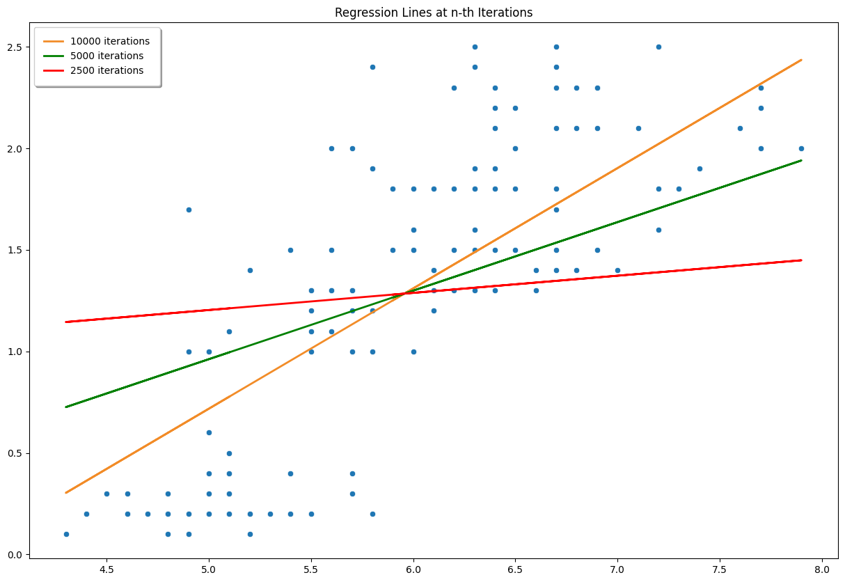

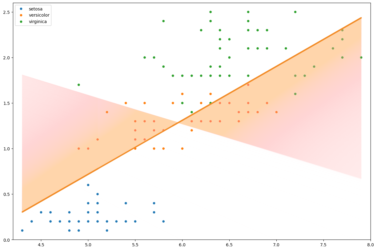
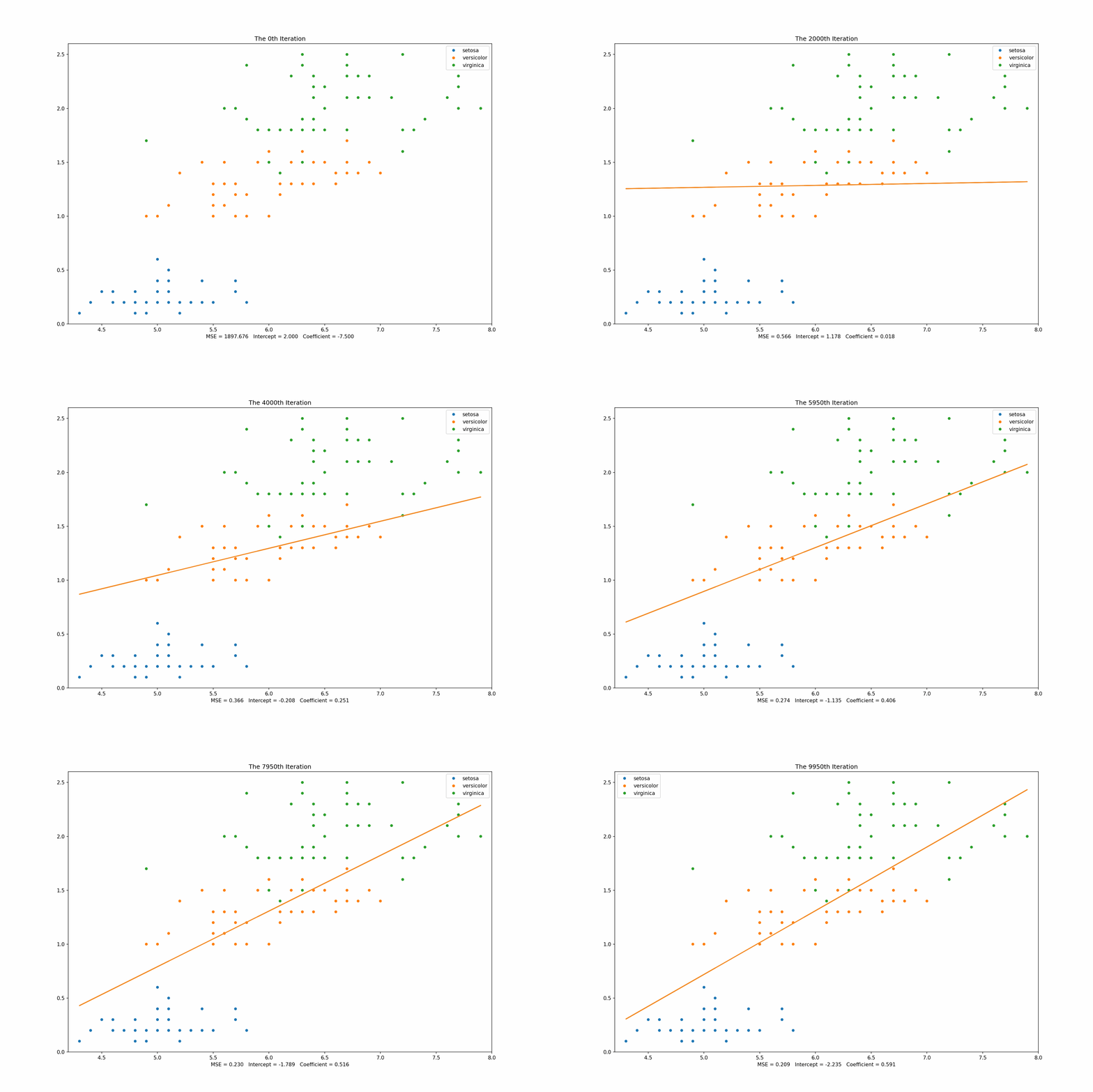
Conclusion

BGD Loss Function Graph

The change of the regression line over time

Regression line animation

From the graph above, we can see that how the regression line changes from the time to time. After $10,000$ iterations, the MSE value of our own Gradient Descent is $0.195$ which is quite close to our baseline, $0.191$.

The pathway of the cost function over the 2D MSE contour

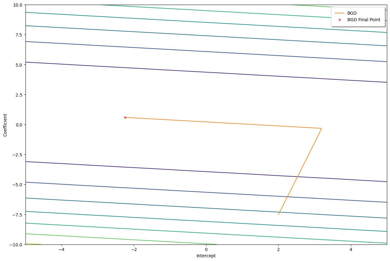
Here are some keypoints for Batch Gradient Descent:

1. Batch Gradient Descent only updates the parameters once after considering all the data points. Thus, it takes longer time for the algorithm to converge.
2. Not only does it takes longer to converge, but it also takes up a lot of computational resources.
3. Batch Gradient Descent is not the best algorithm for large datasets.

Code

def bgd(x, y, epochs, df, alpha = 0.01):
  intercept, coefficient = 2.0, -7.5
  length = len(x)
 
  predictions = predict(intercept, coefficient, x)
  error = predictions - y
  mse = np.sum(error ** 2) / (2 * length)
  df.loc[0] = [intercept, coefficient, mse]
 
  for epoch in range(1, epochs):
    predictions = predict(intercept, coefficient, x)
    error = predictions - y
    intercept_gradient = np.sum(error) / length
    coefficient_gradient = np.sum(error * x) / length
    intercept = intercept - alpha * intercept_gradient
    coefficient = coefficient - alpha * coefficient_gradient
    mse = np.sum(error ** 2) / (2 * length)
    df.loc[epoch] = [intercept, coefficient, mse]
  return df

References

1. Sebastian Ruder. "An overview of gradient descent optimization algorithms." arXiv:1609.04747 (2016).
2. M. Jack. 3D Gradient Descent in Python. Source https://jackmckew.dev/3d-gradient-descent-in-python.html
3. T. Arseny. Gradient Descent From Scratch. Source https://towardsdatascience.com/gradient-descent-from-scratch-e8b75fa986cc
4. O. Artem. Stochastic, Batch, and Mini-Batch Gradient Descent. Source https://towardsdatascience.com/stochastic-batch-and-mini-batch-gradient-descent-demystified-8b28978f7f5
5. P. Sushant. Batch, Mini Batch, and Stochastic Gradient Descent. Source https://towardsdatascience.com/batch-mini-batch-stochastic-gradient-descent-7a62ecba642a
6. Geeksforgeeks. Difference between Batch Gradient Descent and Stochastic Gradient Descent. Source https://www.geeksforgeeks.org/difference-between-batch-gradient-descent-and-stochastic-gradient-descent/
7. Sweta. Batch, Mini Batch, and Stochastic Gradient Descent. Source https://sweta-nit.medium.com/batch-mini-batch-and-stochastic-gradient-descent-e9bc4cacd461
8. Geeksforgeeks. ML | Mini-Batch Gradient Descent with Python. Source https://www.geeksforgeeks.org/ml-mini-batch-gradient-descent-with-python/