Adam

Introduction

Adaptive Moment Estimation (Adam) is an optimization algorithm that is inspired from Adagrad and RMSprop optimization algorithms. Remember that Adagrad and RMSprop have their own limitations.

In the case of Adagrad, the learning rate diminishes over time and becomes too small since the algorithm takes account all of the previous gradients. Thus making the model stops learning.

Even though RMSprop solves the problem of Adagrad by taking account only the average of the previous gradients, it still stuffers from the same problem as Adagrad.

To solve the limitations of Adagrad and RMSprop, Adam introduces the concept of momentum. Let's see how Adam works.

Mathematics of Adam

The parameter update rule is expressed as

where

• $\theta_t$ is the parameter at time $t$
• $\alpha$ is the learning rate
• $\hat{m}_t$ is the corrected first moment estimate
• $\hat{v}_t$ is the corrected second moment estimate
• $\epsilon$ is a small value to prevent division by zero

The corrected first moment estimate is expressed as

where

• $m_t$ is the first moment estimate
• $\beta_1^t$ is the exponential decay rate for the first moment estimate at time $t$
• $g_t$ is the gradient of the cost function at time $t$

The corrected second moment estimate is expressed as

where

• $v_t$ is the second moment estimate
• $\beta_2^t$ is the exponential decay rate for the second moment estimate at time $t$
• $g_t^2$ is the gradient of the cost function at time $t$

It's worth mentioning is that the first moment estimate $m_t$ and the second moment estimate $v_t$ work just like Momentum to maintain directionality since they both take account of the previous gradients. By accumulating previous gradients, Adam accelerates convergence especially in the area with small gradients.

The reason why the first moment estimate $m_t$ has to be corrected is that the first moment estimate $m_t$ is biased to smaller values at the beginning of the training when it is zero or close to zero. The bias could lead to overly aggresive parameter updates, instability, or slow convergence. Similarly with the second moment estimate $v_t$.

Since we only have two parameters, we are going to need $g_{t,0}$ to represent the gradient of the cost function with respect to the intercept, and $g_{t,1}$ to represent the gradient of the cost function with respect to the coefficient. These two can be expressed as follows:

Implementation of Adam

First, calculate the intercept and the coefficient gradient. Notice that the intercept gradient $g_{t,0}$ is the prediction error.

error = prediction - y[random_index]
intercept_gradient = error
coefficient_gradient = error * x[random_index]

Second, calculate the first moment estimate $m_t$ and the second moment estimate $v_t$.

momentum = momentum_decay_rate * momentum + (1 - momentum_decay_rate) * intercept_gradient
variance = variance_decay_rate * variance + (1 - variance_decay_rate) * (coefficient_gradient ** 2)

Third, correct the first moment estimate $m_t$ and the second moment estimate $v_t$.

corrected_momentum = momentum / (1 - momentum_decay_rate ** epoch)
corrected_variance = variance / (1 - variance_decay_rate ** epoch)

Finally, update the intercept and the coefficient.

intercept = intercept - learning_rate * corrected_momentum / (np.sqrt(corrected_variance) + eps)
coefficient = coefficient - learning_rate * corrected_momentum / (np.sqrt(corrected_variance) + eps)

Conclusion

Pathways of Adadelta, RMSprop, and Adam along the 2D MSE contour.

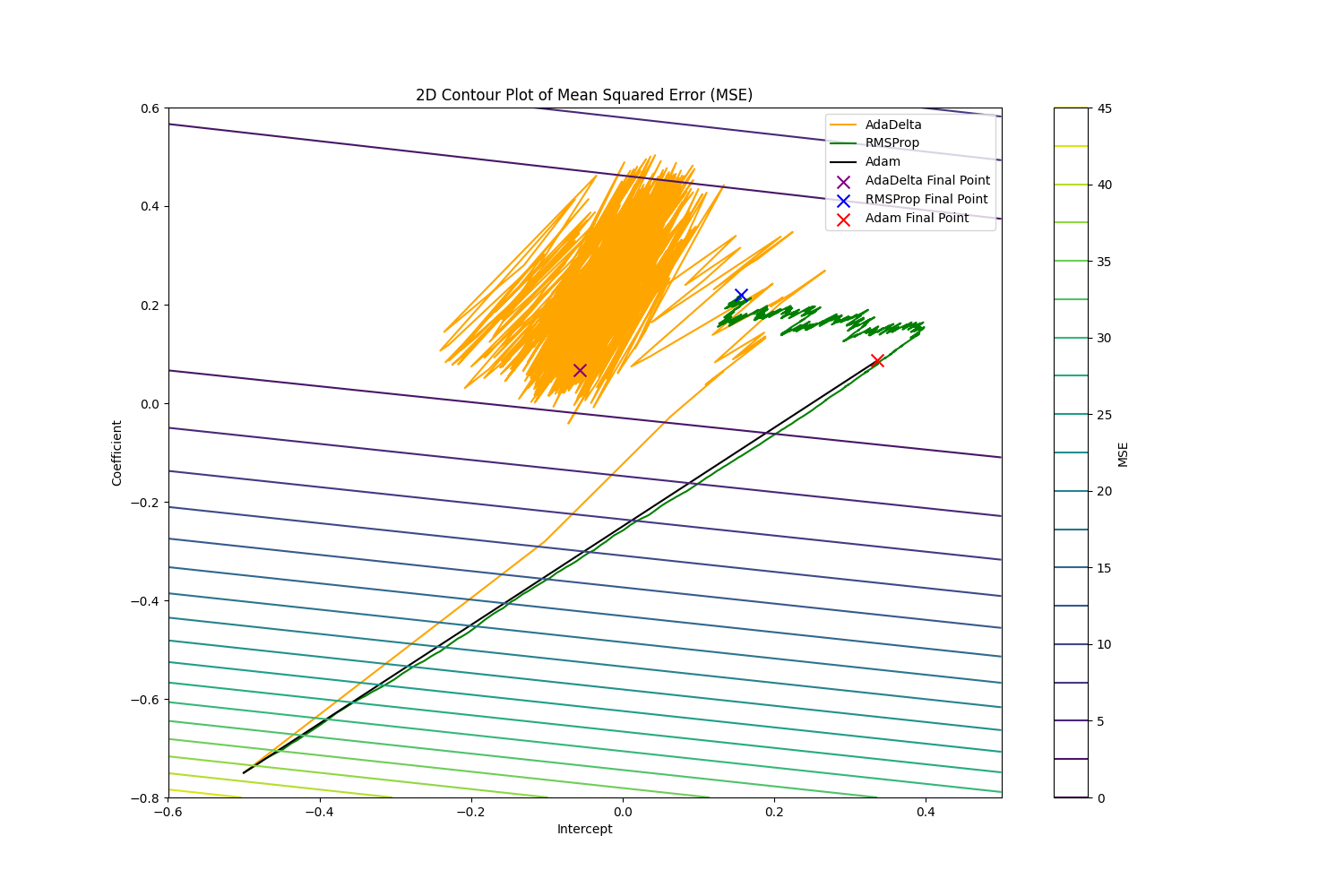
From the figure above, we can see that the pathway Adam took a direct path down the hill compared to the other two. That proves that Adam can accelerate convergence especially in the area with small gradients and avoid frequent updates with the help of Momentum.

Code

def adam(x, y, df, epochs=1000, learning_rate=0.01, eps=1e-8):
  intercept, coefficient = -0.5, -0.75
  momentum_decay_rate, variance_decay_rate = 0.9, 0.999
  momentum, variance = 0.0, 0.0
 
  random_index = np.random.randint(len(x))
  prediction = predict(intercept, coefficient, x[random_index])
  error = prediction - y[random_index]
  df.loc[0] = [intercept, coefficient, momentum, variance, (error ** 2) / 2]
 
  for epoch in range(1, epochs + 1):
    random_index = np.random.randint(len(x))
    prediction = predict(intercept, coefficient, x[random_index])
    error = prediction - y[random_index]
 
    intercept_gradient = error
    coefficient_gradient = error * x[random_index]
 
    momentum = momentum_decay_rate * momentum + (1 - momentum_decay_rate) * intercept_gradient
    variance = variance_decay_rate * variance + (1 - variance_decay_rate) * (coefficient_gradient ** 2)
 
    corrected_momentum = momentum / (1 - momentum_decay_rate ** epoch)
    corrected_variance = variance / (1 - variance_decay_rate ** epoch)
 
    intercept = intercept - learning_rate * corrected_momentum / (np.sqrt(corrected_variance) + eps)
    coefficient = coefficient - learning_rate * corrected_momentum / (np.sqrt(corrected_variance) + eps)
 
    df.loc[epoch] = [intercept, coefficient, corrected_momentum, corrected_variance, (error ** 2) / 2]
 
  return df

References

1. Sebastian Ruder. "An overview of gradient descent optimization algorithms." arXiv:1609.04747 (2016).
2. Diederik P. Kingma, Jimmy Ba. "Adam: A Method for Stochastic Optimization." arXiv:1412.6980 (2014).