SGD with Nesterov

Gradient Descent Algorithm: 11 Part(s)

Introduction

In the previous post about SGD with Momentum, we discussed how Momentum mimics the behavior of a ball rolling down a hill. Thus, it helps in reducing the oscillations and accelerates the convergence of the model. In this post, we will discuss a more efficient version of Stochastic Gradient Descent with Momentum, called Nesterov Accelerated Gradient, which does not blindly following the gradient but also consider the future gradient.

From this now on, I am gonna call Nesterov Accelerated Gradient as NAG.

Mathematics of NAG

The parameter update rule is expressed as

\begin{aligned} v_{i, t} &= \gamma v_{i, t-1} + \alpha \nabla J(\theta_i - \gamma v_{i, t-1}) \\ \theta_i &= \theta_i - v_{0,t} \\ \end{aligned}

where

$v_{i,t}$ is the $i$ -th Momentum vector at time $t$
$\gamma$ is the momentum coefficient
$\alpha$ is the learning rate
$\nabla J(\theta_i - \gamma v_{t-1})$ is the gradient of the cost function at the point $\theta_i - \gamma v_{i, t-1}$ , or the lookahead point
$\theta_i$ is the parameter vector

The gradient of the cost function w.r.t. to the intercept $\theta_0$ and the coefficient $\theta_1$ are expressed as the following.

\begin{aligned} \nabla_{\theta_0} J(\theta) &= \frac{\partial}{\partial \theta_0} J(\theta) \\ &= \frac{1}{2} \frac{\partial}{\partial \theta_0} (\hat{y}_i - y_i)^2 \\ &= \hat{y}_i - y_i \end{aligned}

\begin{aligned} \nabla_{\theta_1} J(\theta) &= \frac{\partial}{\partial \theta_1} J(\theta) \\ &= \frac{1}{2} \frac{\partial}{\partial \theta_1} (\hat{y}_i - y_i)^2 \\ &= (\hat{y}_i - y_i)x_i \end{aligned}

Since there are two parameters to update, we are going to need two parameter update rules.

\begin{aligned} v_{0, t} &= \gamma v_{0, t-1} + \alpha (\hat{y}_i - y_i) \\ \theta_0 &= \theta_0 - v_{0,t} \end{aligned}

\begin{aligned} v_{1, t} &= \gamma v_{1, t-1} + \alpha (\hat{y}_i - y_i)x_i \\ \theta_1 &= \theta_1 - v_{1,t} \end{aligned}

where

\hat{y}_i = \theta_0 - \gamma v_{0, t-1} + (\theta_1 - \gamma v_{1, t-1})x_i

Similar to Momentum, NAG also helps in reducing the oscillations and accelerates the convergence of the model. However, NAG is more "conscience" and efficient than Momentum because it anticipates the future gradient and thus converges faster.

Implementation of NAG

First, calculate the lookahead intercept $\theta_0 - \gamma v_{i, t-1}$ and the lookahead coefficient $\theta_1 - \gamma v_{i, t-1}$ so that we can determine the lookahead prediction.

lookahead_intercept = intercept - gamma * v_intercept
lookahead_coefficient = coefficient - gamma * v_coefficient
 
lookahead_prediction = predict(lookahead_intercept, lookahead_coefficient, x)

Second, determine the value of the gradient of the cost function at the point $\theta_i - \gamma v_{i, t-1}$ , $\nabla J(\theta_i - \gamma v_{i, t-1})$ . Basically, it's the same as the gradient of the cost function w.r.t. to the parameters $\theta_0$ and $\theta_1$ . The only difference is that we are using the lookahead prediction instead of the current prediction.

Notice that the gradient of the cost function w.r.t. to the intercept $\theta_0$ is the prediction error. We can use that to speed up the computation.

error = lookahead_prediction - y[random_index]
t0_gradient = error
t1_gradient = error * x[random_index]

Third, update the Momentum vectors. For simplicity, we are not going to store the vector of $\theta_0$ and $\theta_1$ into a list. Instead, we are storing them into separate variables, t0_vector and t1_vector respectively.

\begin{aligned} v_{0, t} &= \gamma v_{0, t-1} + \alpha \nabla J(\theta_0 - \gamma v_{0, t-1}) \\ v_{1, t} &= \gamma v_{1, t-1} + \alpha \nabla J(\theta_0 - \gamma v_{1, t-1}) \end{aligned}

Since the updated t0_vector relies on the previous t0_vector, we need to initialize them to zero outside the loop.

t0_vector, t1_vector = 0.0, 0.0
...
 
for epoch in range(1, epochs + 1):
  ...
  t0_vector = gamma * t0_vector + alpha * t0_gradient
  t1_vector = gamma * t1_vector + alpha * t1_gradient

Finally, update the parameters.

intercept = intercept - t0_vector
coefficient = coefficient - t1_vector

Conclusion

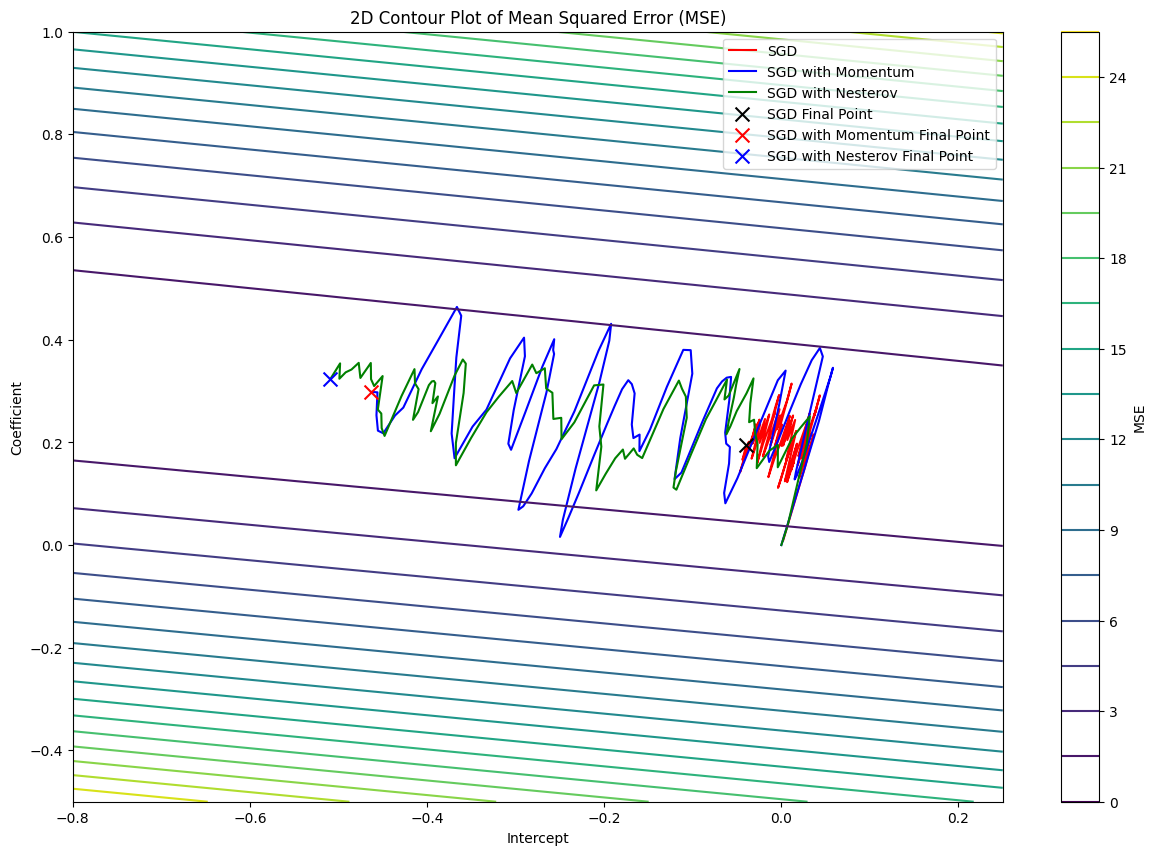The loss function pathways of SGD, SGD with Momentum, and SGD with Nesterov

From the graph above, we can see that NAG oscillates less by anticipating the future gradient unlike Vanilla SGD and SGD with Momentum. The path of the loss function of NAG seems to be more direct and natural, just like a ball rolling down a hill.

Code

def predict(intercept, coefficient, x):
  return intercept + coefficient * x
 
def sgd_nesterov(x, y, df, epochs=100, alpha=0.01, gamma=0.9):
  intercept, coefficient = 0.0, 0.0
  t0_velocity, t1_velocity = 0.0, 0.0
 
  random_index = np.random.randint(len(features))
  prediction = predict(intercept, coefficient, x[random_index])
  error = (prediction - y[random_index]) ** 2
 
  df.loc[0] = [intercept, coefficient, t0_velocity, t1_velocity, error]
 
  for epoch in range(1, epochs + 1):
    random_index = np.random.randint(len(features))
 
    lookahead_intercept = intercept - gamma * t0_velocity
    lookahead_coefficient = coefficient - gamma * t1_velocity
 
    lookahead_prediction = predict(lookahead_intercept, lookahead_coefficient, x[random_index])
 
    t0_gradient = lookahead_prediction - y[random_index]
    t1_gradient = (lookahead_prediction - y[random_index]) * x[random_index]
 
    t0_velocity = gamma * t0_velocity + alpha * t0_gradient
    t1_velocity = gamma * t1_velocity + alpha * t1_gradient
 
    intercept = intercept - t0_velocity
    coefficient = coefficient - t1_velocity
 
    prediction = predict(intercept, coefficient, x[random_index])
    mean_squared_error = ((prediction - y[random_index]) ** 2) / 2
 
    df.loc[epoch] = [intercept, coefficient, t0_velocity, t1_velocity, mean_squared_error]
 
  return df

References

Sebastian Ruder. "An overview of gradient descent optimization algorithms." arXiv:1609.04747 (2016).